Stock-Status Plots (SSPs)

Kristin Kleisner and Daniel Pauly
(full text download)

Stock-status plots are bivariate graphs summarizing the status (e.g., ‘developing’, ‘fully exploited’, ‘overexploited’, etc.), through time, of the multispecies fisheries of a fished area or ecosystem. Given that the limitations of these plots are understood, they are very useful for communicating, at a glance, the evolving status of multispecies fisheries.

Origin of approach

Overfishing occurs in fisheries that have been exploited at levels that exceed the capacity for replacement by reproduction and growth of the exploited species (Ricker 1975; Grainger 1999). Species that are being overfished are producing catches that are below the level that could be sustainably derived. As a result of intense exploitation, most fisheries generally follow sequential stages of development: undeveloped, developing, fully exploited, overfished, and collapsed, with the latter two stages occasionally ameliorated through management action, if management exists and is effective. Building thereon, Grainger and Garcia (1996) conceived the first version of the Stock Status Plots (SSP) by fitting time series of landings with polynomials, and classifying their slopes, i.e.:

1. flat slope at a minimum: undeveloped;
2. increasing slopes: developing fisheries;
3. flat slope at a maximum: fully exploited;
4. decreasing slopes: senescent fishery (collapsed).

This led to the graph reproduced here as Figure 1, which formed the basis for inferences on the status of global fisheries.

Grainger and Garcia’s (1996) main finding was that catch increases were not possible in many cases, and that increased exploitation would result in lower catch rates. This highlighted the fact that even total landings may provide a false sense of security when development phase is not taken into account.

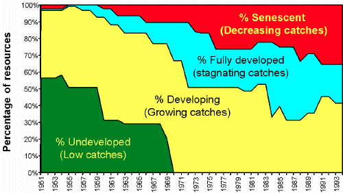
Figure 1. Evolution of the state of world resources from 1950-1994, based exclusively on statistical trends for 200 major stocks (Grainger and Garcia 1996).

Initial streamlining of approach

Froese and Kesner-Reyes (2002), in their analysis of time series of catch data from ICES and FAO with respect to the resilience of species towards fishing, simplified the approach of Grainger and Garcia (1996) by omitting polynomials from their analyses, and designating stock status relative to the historically maximum catch. They defined the fishing status of over 900 stocks as undeveloped, developing, fully exploited, overfished, or collapsed. The designation they used are presented in Table 1.

Table 1. Criteria used to assign development stages to fisheries in FAO production data time series based on Froese and Kesner-Reyes (2002). (‘Catches’ may refer to landings)
Status of fishery	Criterion applied
Undeveloped	Year before maximum catch and catch is less than 10% of maximum value.
Developing	Year before maximum catch  and catch 10-50% of maximum value.
Fully exploited	Catch larger than 50% of maximum value.
Overfished	Year after maximum catch and catch 10-50% of maximum value.
Collapsed/Closed	Year after maximum catch and catch less than 10% of maximum value.

They excluded years 1950 (first) and 1999 (last year of their analysis) because ‘after max. year’ and ‘before max. year’ could not be applied. The typical transition of a fishery from undeveloped through fully exploited, to collapsed or closed is shown in Figure 2. The benefit of this method for interpreting trends in world fisheries was that it did not require fitting polynomial curves to the time series of catches of each stock; hence many more species could be included in analyses (see, e.g., Froese and Pauly 2003). Froese and Kesner-Reyes (2002) also noted that there is a distinct acceleration towards overfished and collapsed status. In addition to increasing losses to the global economy and the livelihoods of millions of people globally, this trend has significant ecological implications: the increasing number of stock collapses and stocks that are overfished point to a decrease in biodiversity. Worm et al. (2006) extrapolated the trend in collapsed fisheries resources to 2048 to show that, assuming continuation of current trends, globally most stocks would experience collapse – a topic that has been hotly debated in the scientific literature.

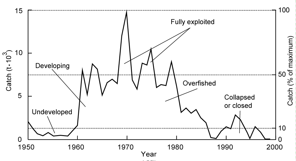
Figure 2. Typical transition of a fishery as illustrated by a time series of catch data transiting from undeveloped through fully exploited, to collapsed, (or closed). See Table 1 for definition of these stages. Modified from a catch time series for the basking shark Cetorhinus maximus in Froese and Kesner-Reyes (2002).

Recent modification and Sea Around Us use

More recently, Pauly et al. (2008) created (and coined the name for) ‘Stock Status Plots’ for a UNEP compendium on Large Marine Ecosystems (LMEs; Sherman and Hempel 2008). They modified the definitions of Froese and Kesner-Reyes (2002) slightly, such as to produce graphs of percentage of stocks by status and percentage catch by stock-status over time (Table 2). One of the main modifications was the combination of the previous categories ‘undeveloped’ and ‘developing’ into a single ‘developing’ category. Pauly et al. (2008) presented stocks as time series of species, genus, or family for which:

1) The first and last reported landings are at least ten years apart;

2) There are at least five years of consecutive catches; and

3) The catch in a particular area (LME) is at least 1,000 tonnes.

Higher taxonomic groupings and pooled groups were excluded. Two plots were created for each LME. The first was a plot of number of stocks by status. To contrast the decline of (stock) biodiversity and bulk catch status, Pauly et al. (2008) also developed a second plot type, i.e., graphs of percentage catch by stock-status over time. These plots, which they called ‘stock-catch status’ plots, jointly with the ‘stock-status’ plots referring to stock numbers, tended to confirm that biodiversity is affected by fishing more strongly than bulk catch.

Table 2. Criteria used by Pauly et al. (2008) to interpret the status of a fishery resource.
Status of fishery	Criterion applied
Undeveloped	Year < max landing AND landing < 10% of max value
Developing	Year < max landing AND landing 10-50% of max value
Fully exploited	Landing > 50% max value
Overexploited	Year > max landing AND landing 10-50% of max value
Collapsed	Year > max landing AND landing < 10% of max value

Kleisner and Pauly (2011) and Kleisner et al. (2013) presented the subsequent development of the original model of Grainger and Garcia (1996) including modifications to make it more usable for the purpose of the Sea Around Us.

One of the critical comments on the previous versions of the stock-status plots was that by definition the percentage of undeveloped or developed stocks was zero in the final year of the time series. To address this, we count stocks that have a peak in catch in the final year of the time series as ‘developing.’ Additionally, we deal with the serious criticism that, in cases where stocks have recovered (e.g., through management actions), the ‘stock- status plots’ do not take stock recovery into account. Norway provides an excellent example of this, e.g., with regards to Atlantic herring, whose catch increased to a maximum in 1966 and then plummeted to a minimum in 1979. Thereafter, the catch gradually increased through the 1980s and early 1990s as a result of management rebuilding actions and remained above 50% of the maximum catch through the 2000s. This recovery should not be reclassified as a ‘developing’ stock; rather an additional category, ‘rebuilding’ (initially labelled as ‘recovering’), is defined when the stock drops to ‘collapsed’ status and then recovers.

To implement this, a ‘post-maximum minimum’ was defined as the minimum landings occurring after the maximum landings. This modification also addresses the former concern that, by definition the percentage of developing stocks is zero in the final year of the time series. Because ‘recovering’ is a form of stock (re-)development (hence now called ‘rebuilding’), it is displayed within the ‘developing’ category in the plots, and thus better demonstrates the amount of improvement in the status of stocks within a particular area (See Figure 3, top).

The final criterion for determining the stocks’ status by area is presented in Table 3. To better view the overall trend and remove anomalous peaks in the stock-catch status plots, we use a three-year running average to smooth the curves.

Table 3. Criteria used to interpret the status of fishery resources based on time series of catch. This requires the definition of a ‘post-maximum minimum’ (post-max. min.): the minimum landing after the maximum catch  Sources: Kleisner and Pauly (2011) and Kleisner et al. (2013).
Status of fishery	Criterion applied
Rebuilding (Recovering)	Year of landing > year of post-max. min. landing AND post-max. min. landing < 10% of max. landing AND landing is 10-50% of max. landing
Developing	Year of landing < year of max. landing AND landing is < or = 50% of max. landing OR year of max. landing = final year of landing
Exploited	Landing > 50% of max. landing
Over exploited	Year of landing > year of max. landing AND landing is between 10-50% of max. landing
Collapsed	Year of landing > year of max. landing AND landing is < 10% of max. landing

The Sea Around Us’ SSPs are created in four steps (Kleisner and Pauly 2011). The first step is the definition of a stock. We define a stock to be a taxon (either at species, genus or family level of taxonomic assignment) that occurs in the catch records for at least 5 consecutive years, over a minimum of a 10 year time span, and which has a total catch in a given area of at least 1000 tonnes over the time span. Secondly, we assess the status of the stock for every year, relative to the peak catch. We define the five states of stock status for a catch time series (Table 3). This definition is assigned to every taxon meeting the definition of a stock for a particular spatial area considered (e.g., EEZ, LME). Thirdly, we create the graph of number of stocks by status by tallying the number of stocks in a particular state in a given year, and presenting these as percentages. Finally, the cumulative catch of stock by status in a given year is summed over all stocks and presented as a percentage in the catch by stock status graph, or stock-catch-status plot (SCSP). The combination of these two figures represents the complete SSP (Figure 3).

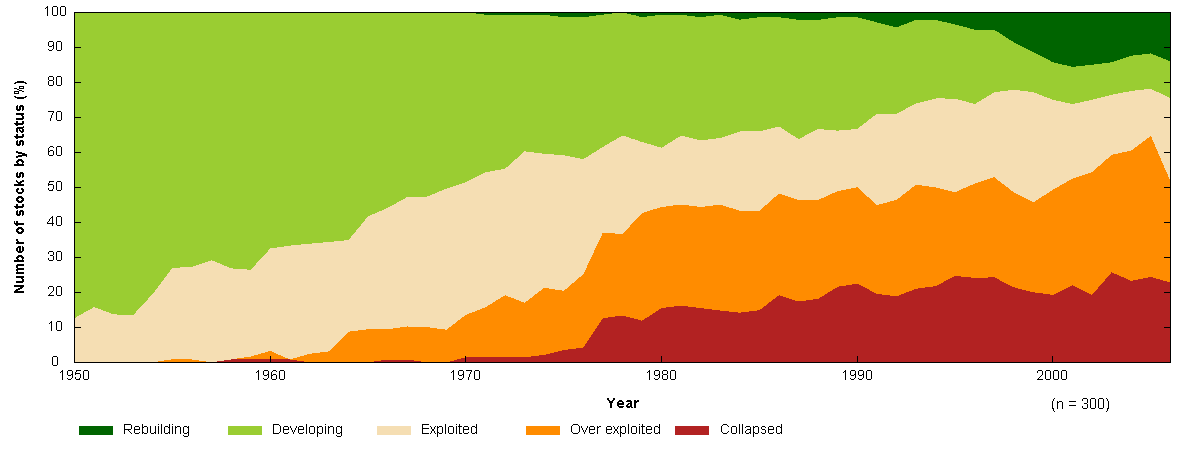
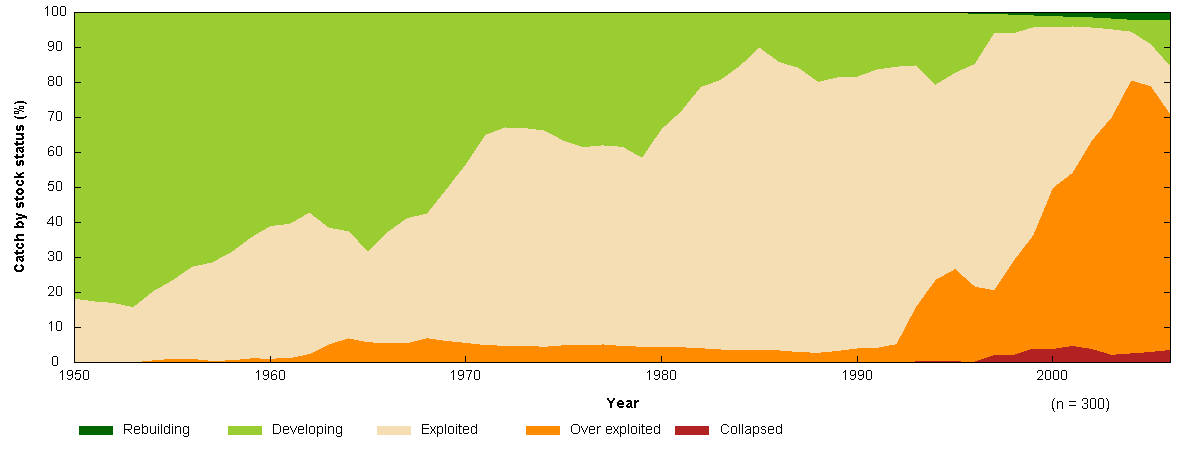
Figure 3. Example of a Stock Status plot as defined by the Sea Around Us for the Kuroshio Current LME; note rebuilding stocks in the upper right corners of the graphs (see text).

The number of stocks by status graph illustrates the (typically increasing) number of stocks that are considered overfished or collapsed. The catch by stock status graph demonstrates that often we are taking the bulk of catches from an increasingly smaller number of stocks, as more stocks become overfished or collapsed. Jointly, these two graphs, and hence the SSP points to an increase in stocks that are compromised, and a decrease in the biodiversity of exploited fishery resources, both in the above example, and in the world in general.

Thus, the stock-status plots as defined here are useful for demonstrating how global fisheries resources have transitioned through the development stages, and the general inability of management to maintain them at an acceptable level of exploitation (Worm et al. 2006). The application of this approach to LMEs and other spatially explicit areas is straightforward. However, the interpretation of the stock-catch status plots can be somewhat problematic due to the fact that they are based on catches and not on population size estimates. Thus, all available additional information sources, such as stock assessments (if available for selected species and stocks), and management history, actions and effectiveness should be considered (see, e.g., Froese et al. 2012, 2013). Despite this, stock-status plots remain a useful tool for visualizing fisheries resource trends at the global level.

References

Froese R and Kesner-Reyes K (2002) Impact of fishing on the abundance of marine species. ICES CM 2002/L: 12, 15 p.

Froese R and Pauly D (2003) Dynamik der Überfischung. pp. 288-295 In: Lozán J, Rachor E, Reise K, Sündermann J and von Westernhagen H (eds.), Warnsignale aus Nordsee und Wattenmeer – eine aktuelle Umweltbilanz. GEO, Hamburg.

Froese R, Zeller D, Kleisner K and Pauly D (2012) What catch data can tell us about the status of global fisheries. Marine Biology 159(6): 1283-1292.

Froese R, Zeller D, Kleisner K and Pauly D (2013) Worrisome trends in global stock status continue unabated: a response to a comment by R.M. Cook on “What catch data can tell us about the status of global fisheries”. Marine Biology 160: 2531-2533.

Grainger RJR (1999) Global trends in fisheries and aquaculture. p. 21-25 In: National Ocean Service, NOAA, Center for the Study of Marine Policy at the University of Delaware, The Ocean Governance Group. 1999. Trends and Future Challenges for US National Ocean and Coastal Policy: Workshop Materials. Washington, D.C.

Grainger RJR and Garcia S (1996) Chronicles of marine fisheries landings (1950-1994): trend analysis and fisheries potential. FAO Fisheries Technical Paper 359, 51 p.

Kleisner K and Pauly D (2011) Stock-Status Plots of fisheries for Regional Seas. pp. 37-40 In: Christensen V, Lai S, Palomares MLD, Zeller D and Pauly D (eds.), The state of biodiversity and fisheries in Regional Seas. Fisheries Centre Research Reports 19(3), University of British Columbia, Vancouver.

Kleisner K, Zeller D, Froese R and Pauly D (2013) Using global catch data for inferences on the world’s marine fisheries. Fish and Fisheries 14(3): 293-311.

Pauly D, Alder J, Booth S, Cheung WWL, Christensen V, Close C, Sumaila UR, Swartz W, Tavakolie A, Watson R and Zeller D (2008) Fisheries in Large Marine Ecosystems: Descriptions and Diagnoses. pp. 23-40 In: Sherman K and Hempel G (eds.), The UNEP Large Marine Ecosystem Report: a Perspective on Changing Conditions in LMEs of the World’s Regional Seas. UNEP Regional Seas Reports and Studies No. 182, Nairobi.

Ricker WE (1975) Computation and interpretation of biological statistics of fish populations. Bulletin of the Fisheries Research Board Canada 191, 382 p.

Sherman K and Hempel G, editors (2008) The UNEP Large Marine Ecosystem report: a Perspective on Changing Conditions in LMEs of the World’s Regional Seas. UNEP Regional Seas Reports and Studies No. 182, United Nations Environment Programme, Nairobi. 852 p.

Worm B, Barbier EB, Beaumont N, Duffy JE, Folke C, Halpern B, Jackson J, Lotze H, Micheli F, Palumbi SR, Sala E, Selkoe KA, Stachowicz JJ and Watson R (2006) Impacts of biodiversity loss on ocean ecosystem services. Science 314(5800): 787-790.