Contents
Exclusive Economic Zones (EEZ)
EEZ area measure
EEZ declaration year
Shelf area
Inshore Fishing Area (IFA)
Coral Reefs
Seamounts
Primary Production
Large Marine Ecosystems
Exclusive Economic Zones (EEZ)
Dirk Zeller and Daniel Pauly
Disclaimer
Maritime limits and boundaries depicted on Sea Around Us maps are not to be considered as an authority on the delimitation of international maritime boundaries. These maps are drawn on the basis of the best information available to us. Where no maritime boundary has been agreed, theoretical equidistance lines have been constructed. Where a boundary is in dispute, we attempt to show the claims of the respective parties where these are known to us and show areas of overlapping claims. In areas where a maritime boundary has yet to be agreed, it should be emphasized that our maps are not to be taken as the endorsement of one claim over another.
Background
Historically, the oceans of the world were considered ‘free’ to anyone wanting to use them for travel, trade or resource exploitation. However, claims to territorial seas date back at least to the 1700s when the Dutch first claimed such an area based on the range of coastal cannon batteries, which, at the time, reached at most three nautical miles (nm). Thus, the three-mile territorial seas concept was born.
Countries have ever since tried to exert control over parts of the ocean that border their shores, as maritime boundaries and claims can have significant impacts on many marine activities, including ownership of living and non-living resources and fishing access. The United Nations Convention on the Law of the Sea (UNCLOS), initiated in the 1960s, established a framework that permitted countries to define their claims over ocean areas, and provided agreed upon definitions for territorial seas (now defined as 12 nm), contiguous zones (24 nm, for prevention of infringements of customs, fiscal, immigration and sanitary regulations) as well as 200 nm Exclusive Economic Zones (EEZ), which now cover most shelf areas. Most countries declared EEZs after the completion of the Convention and the subsequent adoption of UNCLOS as international law. Within its EEZ, a country has the sovereign right to explore and exploit, conserve and manage living and non-living resources in the water column and on the seafloor, as defined by Part V of the Law of the Sea.
The Law of the Sea also makes allowances, through the Commission on the Limits of the Continental Shelf, for countries to claim extended jurisdiction over shelf areas beyond 200 nm, if they can demonstrate that their continental shelf extends beyond the established 200 nm EEZ. Note that this does not extend national jurisdiction over fisheries resources per se, but rather seafloor resources such as oil and gas and seafloor mining. National claims for EEZs and extended jurisdiction may overlap, creating areas of disputed ownership and jurisdiction. Settlements through boundary agreements may take many years to develop and are complex, resulting in numerous disputed areas and claimed boundaries.
What is the data source for maritime boundaries used by the Sea Around Us?
The EEZ boundaries we use in our database were adapted from the public domain ‘Maritime Boundaries Geodatabase’ available from the Flanders Marine Institute (VLIZ, Belgium), now available via www.marineregions.org, overlaid onto the ½ degree x ½ degree spatial cells mapping system of our database. Given the ½ x ½ degree nature of our spatial mapping system, area measurements of EEZs based on our data may differ slightly from those of other systems, and should be considered approximations. Note also that we deal with major disputed areas and unsettled boundary disputes by presenting the areas as ‘disputed areas’ with reference to those countries involved in the claim. We welcome information for improvements and corrections, as well as negotiated agreements on settlement of disputed areas.
Also note that
- some countries (e.g., around the Mediterranean) have not declared EEZs, in which case we defined EEZ boundaries for these countries based on data and the general methods used by the Flanders Marine Institute, as if these countries were to apply the UNCLOS rules to their definitions; and
- some countries (notably European Union member states) do not use EEZ for fisheries management.
EEZ area measure
Surface areas are expressed in km2 and were obtained by overlaying a global 2-minute cell ESRI GRID of surface area values with a matching ESRI GRID of EEZs. For each EEZ the intersecting surface area based on the 2-minute raster was extracted and summed. Thus, area measure may differ from national area measures countries may derive from detailed in-situ measurements using legally defined baselines. Furthermore, while the legal definition of EEZs begins at the territorial seas boundary, we conceptually include territorial seas (generally up to 12 nm from shore) within our EEZs, as 12 nm territorial areas are generally too small to differentiate at the scale of our global ½ degree cell grid system.
EEZ declaration year
Each EEZ in the Sea Around Us database is assigned an ‘EEZ declaration year’. This reflects the year in which this EEZ was officially declared by a country, or in cases where no EEZ was declared (or the exact date could not be ascertained), we took the year 1982 (conclusion of the UNCLOS convention) as the assumed declaration year. For years prior to the declaration year, we treat these EEZ-equivalent waters as ‘open access’. This open access is, however, modified in cases where we have explicit knowledge of a distant water country fishing or not fishing in a given EEZ during these earlier years. For all years after the EEZ declaration year, an access agreement or an observed access as per the Sea Around Us access databases is required for foreign catches to be allocatable to the given EEZ.
Shelf area
Dirk Zeller and Daniel Pauly
Continental shelves are the submarine continental landmass that extends from the shore line (intertidal area) offshore, resulting in an area of relatively shallow water (usually < 200 m) known as the shelf area. UNCLOS legally defined the continental shelf as the stretch of the seabed adjacent to the shores of a particular country to which it belongs.
The Sea Around Us defines shelves as continental shelf areas from shore to a depth of 200 m. Thus, the area of each ‘shelf’ was prepared in a similar manner to EEZ area, but was truncated at 200 m depth, i.e., at the shelf edge, based on the United States National Geophysical Data Center’s ETOPOS GLOBAL 2’ ELEVATION data.
Inshore Fishing Area (IFA)
Dirk Zeller and Daniel Pauly
Our reconstructed catch data define catches by fishing sector, and make a major distinction between large-scale (i.e., industrial) fisheries catches, and small-scale (i.e., artisanal, subsistence and recreational) fisheries catches. This distinction, besides being based on type and size of vessels and fishing gears used for fishing, also includes a spatial component in our definition. Thus, while industrial fisheries can have access to all waters within and outside EEZs, we define all small-scale fisheries as being restricted to more inshore, coastal waters. Therefore, we make use of the Inshore Fishing Area (IFA) concept as defined by Chuenpagdee et al. (2006), who defined IFA as: the area that extends from shore to either 50 km offshore or to the 200 m depth contour, whichever comes first. We amend this definition slightly: only territories that are inhabited and have local fisheries are defined as having an IFA. Thus, uninhabited territories, such as many sub-Antarctic islands, which are not inhabited (or only host government employees as part of research or meteorological stations) do not have IFAs. The areas in km2 are measured similar to EEZ and shelf areas.
Reference
Chuenpagdee R, Liguori L, Palomares MD and Pauly D (2006) Bottom-up, global estimates of small-scale marine fisheries catches. Fisheries Centre Research Reports 14(8), University of British Columbia, Vancouver. 112 p.
Coral Reefs
Daniel Pauly
Tropical coral reefs, along with tropical rainforests, are the most diverse ecosystems on earth. They contain a multitude of species connected through a myriad of complex feeding and behavioral interactions that are still being unraveled. The bulk of these interactions involve coral reef fishes and invertebrates, here made accessible on a per-country basis using FishBase (www.fishbase.org) and SeaLifeBase (www.sealifebase.org).
Coral reefs generally do not occur in deep waters; most live between the water surface and about 30 m, as established by Charles Darwin in the 1830s. Yet, the surface area covered by coral reefs in various parts of the world has long been a matter of controversy. One of the first estimates was by Newell (1971), but it was so uncertain (150,000-1,500,000 km2) as to be nearly useless. Smith (1978) presented the first credible estimates, which were divided into nine zones, ranging from the South Atlantic, with 8,000 km2, to Southeast Asia with 182,000 km2.
Other estimates followed, again ranging from very low (112,000 km2; De Vooys 1979) to very high (1,994,000 km2; Cooper 1994). Spalding and Grenfell (1997) identified the source of discrepancy between these estimates as issues of definition (‘what is a coral reef?’) and issues of scale (‘what maps are used to identify coral reefs?’). They also provided their own estimate of 255,000 km2, which was near the lower range of previous estimates.
We abstain from presenting country specific coral reef area estimates in absolute terms. Rather, we have interfaced the coral reef maps of the World Conservation Monitoring Centre (www.unep-wcmc.org) with the definitions of Exclusive Economic Zones (EEZ) used for other products of the Sea Around Us to calculate the fraction of the world’s global coral reef area that occurs in the EEZ, or part thereof, of a given country. To obtain absolute surface areas, users can thus multiply this percentage by their preferred estimates of the global surface area covered by coral reefs.
We are aware that this procedure will lead only to approximate values, as certain countries may boast more of certain types of corals than others, which, via one’s definition of coral reefs, might influence what one perceives as coral reef coverage. The problem here, however, is not the absolute amount of coral reef cover, but the fact that terrigenous pollution, overfishing, coral extraction, and global warming, have much reduced live coral cover in most countries, and will increasingly do so in the next decades. Thus our percentages indicate, for each country, the fraction of the problem that each country ought to resolve.
References
De Vooys CGN (1979) Primary production in aquatic environments. In: B Bolin, ET Degens, S Kempe and P Ketner (eds.) SCOPE, 13: The global carbon cycle. John Wiley and Sons. Chichester, UK.
Newell ND (1971) An outline history of tropical organic reefs. American Museum Novitates 2465: 1-37.
Smith SV (1978) Coral reef area and the contributions of reef to processes and resources of the world’s oceans. Nature 273: 225-226.
Spalding MD and Grenfell AM (1997) New estimates of global and regional coral reef areas. Coral Reefs 16: 225-230.
Seamounts
Adrian Kitchingman, Sherman Lai and Daniel Pauly
Introduction
Seamounts are undersea mountains (usually of volcanic origin) rising from the seafloor and peaking below sea level (Duxbury and Duxbury 1989; Kennish 2000). Typically, seamounts are formed by volcanic activity over hotspots in the earth’s crust (Epp and Smoot 1989). Spreading of the sea floor away from these hotspots via plate tectonic movements means that seamounts often form long chains or elongated clusters. There are many opinions on what defines a seamount, but one widespread definition states that a seamount should be steep-sided and rise 1,000 m or more from the sea floor (Duxbury and Duxbury 1989; Epp and Smoot 1989). The shape of seamounts is also an important factor, often crucial in the identification of seamounts from sea floor data. Most are circular or elliptical (Epp and Smoot 1989), although very elongated seamounts do occur (Wessel and Lyons 1997).
While seamounts are relatively common, global seamount datasets containing information on seamount positions are rare and often only contain data for single oceans (e.g., Fornari et al. 1987; Smith and Jordan 1988; Epp and Smoot 1989; Smith and Cann 1990; Wessel and Lyons 1997). In fact, Wessel and Lyons (1997) state that despite the post-World War II increase in oceanographic exploration, only a small fraction of seamounts have actually been mapped bathymetrically. Any detailed global seamount datasets that exist are usually maintained by governmental departments and are not available to the public. We have conducted a global analysis to generate a spatial dataset of points across the world’s oceans that indicate large peaked bathymetric anomalies with a high probability of being seamounts, and the resultant ‘seamount’ database is incorporated into the Sea Around Us collection of databases and web-products.
Obtaining data on seamounts has taken many forms over the years, ranging from visually scanning contour maps (Batzia 1982) to extrapolating using remote sensing data (Wessel 1997). Here, the bathymetric data contained in the ETOPO2 1 raster dataset supplied by NOAA was chosen as the baseline data from which possible global seamount locations were inferred.
For the purpose of the Sea Around Us, a global database of seamount point locations was required, and thus we generated, at least, a lower estimate of the number of seamounts in the world’s oceans.
Methods
The criteria used to study seafloor anomalies across the globe were more general than the vertical gravity gradients used by Wessel (1997), or the slope and length to width ratios used by Batzia (1982). We assumed that a possible seamount should have a rise of 1,000 m or more from the seabed and should be roughly circular or elliptical in shape. Moreover, since the ETOPO2 data were the source for all analyses, the occurrence of volcanic activity was not a defining parameter.
The ETOPO2 dataset was constructed from a variety of sources, but mainly consists of data from satellite altimetry. The dataset was supplied at a 2-minute cell resolution (13.7 km2 at the equator), which allowed a generalized, global analysis, but likely resulted in seamounts being missed.
The ESRI ArcGIS2 software flow direction and sink algorithms (ArcGIS) were used in combination with the ETOPO2 data to obtain the locations of all detectable peaks on the sea floor. The ETOPO2 data was used in an ESRI grid format for a cell-by-cell analysis.
The ETOPO2 elevation data was prepared by first eliminating all land cells (any elevation above 0 m mean sea-level) and then converting negative elevation values to absolute numbers. This allowed using the ESRI algorithms (see below), designed to detect downhill flow direction and sinks, to identify, in our case, the equivalent of uphill flow direction and peaks.
The ESRI flow direction algorithm was first applied to the ETOPO2 data, producing a grid in which each cell is allocated a flow direction value determined by the steepest descent from the immediate surrounding cells. There are eight valid flow direction values indicated in Figure 1. For example, if a focus cell’s direction of steepest slope is to the right, the focus cell’s value is 1.
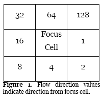
Cells determined to have an undefined flow direction were given a value equal to the sum of the possible flow direction values. Undefined flow directions occurred when all surrounding cells are higher than the focus cell or when two adjacent cells flow into each other. The ESRI sink algorithm was used on the resulting flow direction grid to identify all flow direction cells that have undefined flow directions. The resulting sink (seafloor peak) grid could then be overlaid with the ETOPO2 depth grid to indicate all identifiable peaks on the sea floor.
Using the detected peaks, two methods were used to identify possible seamounts. The first involved isolating peaks found associated with a significant rise from the ocean floor. The second method isolated peaks with a circular or elliptical base in an effort to eliminate small peaks found along steep ridges. The overlapping peaks found by using both of these methodologies were used as the project’s potential seamount dataset. To determine the overlap in the datasets generated from the two methods, points had to be within 2 minutes of each other.
Method 1
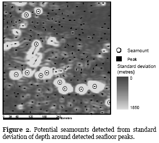
The initial process involved producing a grid of standard deviation of depth across the ocean floor. The neighborhood statistics function in ESRI’s ArcGIS Spatial Analyst software was used to produce a grid giving a standard deviation in depth value for each ETOPO2 depth cell as compared to its immediate neighborhood.
In order to enable the identification of possible seamounts, the standard deviation and seafloor peak grids were overlaid. Using ESRI’s ArcGIS Spatial Analyst, each peak cell was then compared to a 5 x 5 kernel of its neighbourhood on the standard deviation grid. If any cells within the block were above a 300-meter standard deviation, the focal peak cell was considered a possible seamount (Figure 2).
Method 2
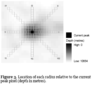
The second method used the peak grid dataset in comparison to the ETOPO2 depth data. An algorithm was developed that scanned ETOPO2 depths around each peak, along 8 radii of 90 km each, at 45o intervals (Figure 3). The lowest and highest depths over the radii (10 cells per radii near the equator, more at higher latitudes) were then recorded. A raw peak was considered a seamount when the following conditions were met:
- Each and all of the 8 radii included depths differing by at least 300 m. This helped eliminate insignificant seamounts;
- If 2 radii included depths between 300 m and 1,000 m, with the shallowest point being closer to the peak than to the deepest point, and if the radii formed an angle of less than 135o. This condition was used to help eliminate ridges from seamounts; and
- At least 5 of the 8 radii around a peak included depths with a difference of a least 1,000 m, with the shallowest point being closer to the peak than to the deepest point.
Results
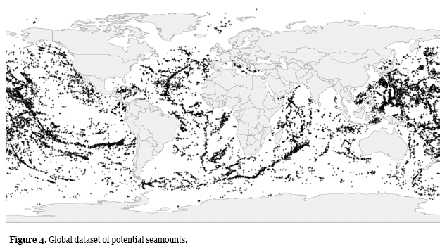
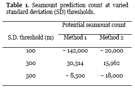
The two methods produced different numbers of potential seamounts, with the first method producing almost twice as many potential seamounts (30,314) as the second method (15,962). Using an overlap method for the two derived datasets, the overlapping points identified 14,287 possible seamounts (Figure 4, see also Kitchingman et al. 2007). The 300-meter standard deviation threshold, used in the first method, produced seamounts that were within the broad seamount definition. As expected, many of the predicted seamounts occurred along mid-ocean ridges.
The range of seamount numbers varied differently for the two methods and their set thresholds. Smaller potential seamounts were identified by Method 1 when the standard deviation threshold was lowered, thus increasing the seamount count (Table 1). Method 2 remained relatively constant, with estimates between 15,000 and 20,000 seamounts depending on depth change threshold set between 100 m and 500 m. The non-linear variation in seamount counts as the threshold is increased for Method 2 is attributed to the fact that the proximity to the nearest seafloor rise and the depth of the valley between is taken into account as well as the change in surrounding depth (Table 1).
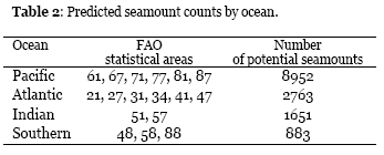
‘Ground truthing’ was performed on a dataset of known seamounts at a 30-minute resolution and produced from a combination of data from the US Department of Defense Gazetteer of Undersea Features (1989) and SeamountsOnline (http://seamounts.sdsc.edu). It was found that approximately 60% of the known seamounts were within 30 minutes of predicted seamounts. Since many studies are restricted to a particular ocean, an attempt to get an estimate of predicted seamounts per ocean was performed (Table 2). The United Nations Food and Agriculture Organization (FAO) statistical areas were used to identify oceans. The seamount count for the Pacific Ocean falls within the bounds of Wessel’s (1997) estimate of 8,882.[1] However, it is still below predictions of 12,000 by Batzia (1982), who also stated the probability of 22,000 to 55,000 seamounts in the Pacific Ocean. Counts differ according to the boundary definitions of the Southern Ocean. The defining FAO areas would have underestimated the actual coverage of the Southern Ocean.
Discussion
We present a relatively simple method for extrapolating potential seamounts from mid-resolution bathymetric data. Although there is no reference to volcanism, the requirement for finding large undersea peaked features (potential seamounts) was fulfilled. The criteria for the extrapolation was only sensitive to a broad level, with the definition of seamounts still very generalized. This sensitivity is also directly influenced by the depth standard deviation threshold and the scope of the neighbourhood cells examined (Method 1) or length of radii (Method 2). The sensitivity of the extrapolation is also directly influenced by the resolution of the underlying bathymetry data. Any features smaller than the cell size of the bathymetry data will have their dimensions blurred with surrounding features, which could bring them outside the bounds of extrapolation criteria.
The ranges in the number of the potential seamounts predicted by both methods are caused by the actual task performed by each method. Method 1 detects the degree of change in depth surrounding a detected peak. The wider the degree of change permitted, the smaller the potential seamounts that can be located. Method 2 was used to identify the peaks that had surrounding depth profiles conforming to the general shape of a seamount (circular or elliptical). Although the depth change ranges could be altered for Method 2, only a limited number of seamounts conformed to our criteria, regardless of the depth change threshold. Our attempt to eliminate peaks along ridges could also eliminate actual seamounts. This leads to the conclusion that the criteria used by Method 2 are too restrictive. It was decided to keep the results conservative (i.e., find only very obvious seamounts) in order to reduce error. The results were also restricted by both methods in the scope of the area around each peak was tested for seamount characteristics. The kernel used by Method 1 equates to an area of approximately 342 km2 at the equator. It was hoped that a kernel of this size would allow the detection of large seamounts while eliminating large peaked banks. This kernel size could be further looked into in order to optimize the analysis sensitivity. Likewise the radii lengths in Method 2 have a similar effect and could also be optimized. Our methodology has provided a relatively simple way of generating a global seamount dataset directly from elevation data (Figure 4).
Although the current output is suitable for fisheries-related global analyses, tighter seamount predictions should be possible with some refinements to the methods used. The set of location data generated here (see Appendix 1 of Kitchingman and Lai 2004) should be considered a subset of a much larger global set of seamount locations, as 50,000 or more seamounts could be identified using bathymetric maps of higher resolution that are presently classified, combined with a broader definition of seamounts, which would take into account the true extent of their variety in shape and groupings.
References
Batzia R (1982) Abundances, distribution and sizes of volcanoes in the Pacific Ocean and implications for the origin of non-hotspot volcanoes. Earth and Planetary Science Letters 60: 195-206.
Duxbury AC and Duxbury AB (1989) An Introduction the World’s Oceans (2nd Edition). William C. Brown Publishers, Dubuque, Iowa.
Epp D and Smoot NC (1989) Distribution of Seamounts in the North Atlantic. Nature 337: 254-257.
Fornari DJ, Batiza R and Luckman MA (1987) Seamount abundances and distribution near the East Pacific Rise 0°-24°N based on seabeam data. Pp. 13-21 In: Keating B, Fryer P, Batiza R (eds.). Seamounts, Islands, and Atolls. American Geophysical Union, Washington, D.C.
Kennish MJ (ed.) (2000) Practical Handbook of Marine Science. Third Edition. CRC Press, New York.
Sandwell DT, Müller RD, Smith WHF, Garcia E and Francis R (2014) New global marine gravity model from CryoSat-2 and Jason-1 reveals buried tectonic structure. Science 346: 65-67.
Smith DK and Cann JR (1990). Hundreds of small volcanoes on the median valley floor of the Mid-Atlantic Ridge at 24-30° N. Nature 348: 152-155.
Smith DK and Jordan TH (1988) Seamount Statistics in the Pacific Ocean. Journal of Geophysical Research 93(B4): 2899-2918.
Stocks K (2004) Seamount invertebrates: composition and vulnerability to fishing. Pp. 17-24 In: Morato T and Pauly D (eds.). Seamounts: Biodiversity and Fisheries. Fisheries Centre Research Reports 12(5), University of British Columbia, Vancouver.
US Department of Defense (1989) Gazetteer of undersea features. CD-ROM, US Department of Defense, Defense Mapping Agency. USA.
Wessel P (1997) Sizes and ages of seamounts using remote sensing: Implications for intraplate volcanism. Science 277: 802-805.
Wessel P (2001) Global distribution of seamounts inferred from gridded Geosat/ERS-1 altimetry. Journal of Geophysical Research 106(B9): 19431-19441.
Wessel P and Lyons S (1997) Distribution of large Pacific seamounts from Geosat/ERS-1: Implications for the history of intraplate volcanism. Journal of Geophysical Research 102(B10): 22459-22475.
Primary Production
Kristin Kleisner and Chris Hoornaert
Background
Primary production (PP) is the fixation of inorganic carbon by living organisms, leading to the formation of organic compounds. Most of the world’s PP relies on energy provided by sunlight, i.e., on the process of photosynthesis. In the deep sea, however, some PP is based on different chemical processes. While seagrasses, macroalgae, and coral reefs (mainly through zooxanthellae that live in a symbiotic relationship with corals) contribute significantly to PP in coastal zones, especially in the tropics, the bulk of marine PP is carried out by microscopic, planktonic algae (‘phytoplankton’), which, in aggregate, can be seen from space, thanks to their photosynthetic pigments (mainly chlorophyll).
Data source
The PP estimates that form part of the Sea Around Us databases are based on a model described by Platt and Sathyendranath (1988), whose parameterization varies between biomes and biogeochemical provinces (Longhurst et al. 1995, Hoepffner et al. 1999). The model estimates depth integrated PP based on chlorophyll pigment concentration as derived from SeaWiFS (http://seawifs.gsfc.nasa.gov/SEAWIFS.html) data, and photosynthetically active radiation calculated as in Bouvet et al. (2002).
The PP estimates were processed at the Inland and Marine Waters Unit (IMW), Institute for Environment & Sustainability, EU Joint Research Center (JRC), Ispra, Italy, under the responsibility of Nicolas Hoepffner (nicolas.hoepffner@jrc.it) and Frédéric Mélin (fredreric.melin@jrc.it), and made available on a monthly basis for the 10-year period from 1998-2007 with a spatial resolution of 9 km.
These data were used here to derive estimates of PP for the EEZ of the maritime countries of the world, and other areas of the world ocean, following application of an interpolation procedure, described below, to fill in missing data points in the data set.
Interpolation
The model for estimating primary productivity relies on monthly estimates of chlorophyll and sunlight for any spatial cell of the oceans. One of these parameters was missing in a number of cases, e.g., due to clouds during satellite passages. The interpolation method developed to fill the gaps in the monthly maps aims to avoid some of the deficiencies of standard interpolation methods (i.e., kriging and spline-based methods). Such methods cannot be used because they would tend to underestimate missing costal data, while standard inverse distance methods tend to ‘fade away’ over large areas with missing data.
Our interpolation method first draws a circle around a cell to be interpolated, with 8 radii, at 45 degrees intervals, and a length of 12 cells; I to VIII (Figure 1). Up to 8 non-empty cells between two radii that are closest to the central cell are identified (e.g., A1 and A2 between the radii I/II and V/VI respectively). An estimate of the central value is obtained by taking the mean between each of the available pairs. The mean of the resulting four (or less) estimates is taken as an estimate of the missing central value.
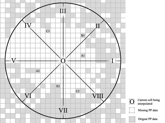
Figure 1: Schematic representation of the interpolation method used to fill in gaps in the cell-specific estimates of primary production. Roman numerals identify the radii between which the filled cells closest to the central missing value cell (e.g., A1 between radii I and II and A2 between V and VI etc.) are located.
Figure 2 gives an example of our completed cell-filling procedure. As expected, PP estimates were missing mainly in the polar regions, and areas with high cloud cover and/or aerosol loads (e.g., the Arabian Sea and northwest Africa). Note that the interpolation method cannot generate estimates higher than the highest observed value. Thus, the high PP values near the poles are not an artifact of the interpolation method.
Some areas with empty cells were larger than the threshold distances (12 cells; see above), which prevented the interpolation procedure from completely filling in the missing values. In these cases, we interpolated between months, and then re-applied the interpolation procedure.
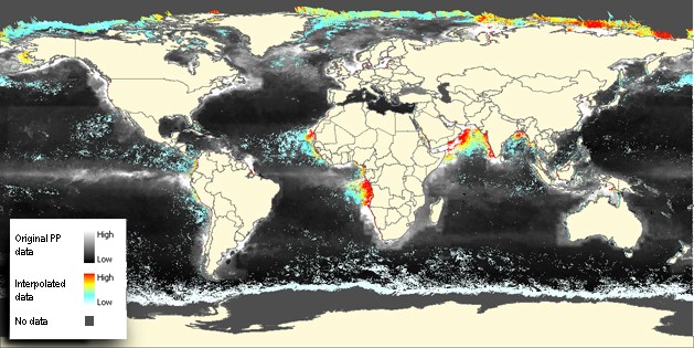
Figure 2: SeaWiFS map of global primary production for June 1998, distinguishing areas with original data from areas with interpolated data. Note large areas without data in the polar regions.
PP as 10-year monthly average for the EEZ of maritime countries, LME or High Sea areas
Estimation of PP for specific areas was achieved by summing cell-specific values in a given area using the 10-year monthly average, and dividing by the total area (water area of each cell), based on GIS objects representing the Exclusive Economic Zone (EEZ) of maritime countries (by FAO areas), Large Marine Ecosystems, or High Sea areas (those parts of FAO statistical areas outside of countries’ EEZ).
This mapping process caused, in some cases, the loss of some fine scale data. This however, affected only countries/territories with an extremely small EEZ, i.e., Bosnia and Herzegovina, or Jordan. In these cases, and for two other countries with small EEZ and unrealistic estimates of PP (Republic of Congo; Democratic Republic of Congo, possibly due to the turbidity of their coastal waters), the original monthly PP estimates were replaced by values averaged from adjacent cells.
References
Platt T and Sathyendranath S (1988) Oceanic primary production: estimation by remote sensing at local and regional scales. Science 241: 1613-1620.
Longhurst A, Sathyendranath S, Platt T and Caverhill C (1995) An estimate of global primary production in the ocean from satellite radiometer data. Journal of Plankton Research 17(6): 1245-1271.
Bouvet M, Hoepffner N and Dowell MD (2002) Parameterization of a spectral solar irradiance model for the global ocean using multiple satellite sensors. Journal of Geophysical Research 107(C12): 8-1 – 8-18.
Hoepffner N, Finenko Z, Sturm B and Larkin D (1999) Depth-integrated primary production in the eastern tropical and sub-tropical North Atlantic basin from ocean colour imagery. International Journal of Remote Sensing 20: 1435-1456.
Large Marine Ecosystems
Daniel Pauly and Dirk Zeller
Large Marine Ecosystems (LMEs) are relatively large ocean areas, adjacent to the continents, and generally in coastal waters where primary productivity is usually higher than in open ocean areas. In cooperation with the University of Rhode Island, NOAA developed the Large Marine Ecosystem (LME; see http://lme.edc.uri.edu/) concept over 30 years ago as a model to implement ecosystem approaches to assessing, managing, recovering, and sustaining LME resources and environments. Today there are 64 LMEs officially defined globally, and NOAA’s LME Program continues to support this important and unique international initiative (see http://lme.edc.uri.edu/). There are considerations under-way to bring this to a total of 66 LMEs due to some splitting of existing, arctic LMEs. The Sea Around Us has already implemented these splits and thus presents 66 LMEs. The LMEs are centers of production, coastal ocean pollution and nutrient overenrichment, habitat degradation (e.g., sea grasses, corals, mangroves), overfishing, biodiversity loss, and climate change effects.
LMEs and fisheries
Traditionally, fisheries have been seen as local or national affairs, largely defined by the range of the vessel exploiting a given resource (Pauly and Pitcher 2000). The need for countries to manage all fisheries within their Exclusive Economic Zones (EEZs), a consequence of the United Nations Convention on the Law of the Sea (UNCLOS), led to attempts to derive indicators for marine fisheries and ecosystems at the national level (see e.g., Prescott-Allen 2001). Also, it was realized that, given the large-scale migration of some exploited stocks, and of distant-water fleets (Bonfil et al. 1998), an even better integration of fisheries could be achieved at the level of Large Marine Ecosystems (LMEs, Sherman et al. 2003, Sherman and Hempel 2008).
However, no national or international jurisdiction reports, at the LME level, catches and other quantities from which fisheries sustainability indicators could be derived. Indeed, if the fisheries of LMEs are to be assessed, and if comparisons of the fisheries in, and of their impact on LMEs, are to be performed, then the fisheries within LMEs must be assembled for this explicit purpose, mainly by assembling data sets pertaining to the EEZs of maritime countries. The only exception to this is the Antarctic LME, for which fisheries catches were mainly provided by the Convention on the Conservation of Antarctic Marine Living Resources (CCAMLR, see Ainley and Pauly 2013).
Thus, the Sea Around Us uses its spatially assigned data (globally assigned to ½ x ½ degree cells) to assemble data on all the fisheries that impact on a given LME (Pauly et al. 2008). The LME framework, thus populated with relevant and current catch and related fisheries data, is set to provide the information needed to develop policies for ecosystem-based fisheries management. It provides a neutral platform for jurisdictions (national and sub-national) to come together to discuss resource management issues as a single ecological unit and look at the consequences of policies, irrespective of boundaries. This information will also provide guidance on information gaps (e.g., spatial effort data) and areas for research (e.g., large-scale fisheries-independent biomass estimation), so that ecosystem based management of fisheries and marine areas can be strengthened in many of the world’s coastal regions.
The LME system can also enhance the global assessments of marine areas and resources. Until recently, large-scale assessments have primarily focused on ocean basins (Pauly et al. 2005) or FAO Statistical Areas (Pauly et al. 1998). However, these are large areas, and the important differences needed for developing policy can be lost in such a large-scale management unit. Assessments based on LMEs can give much better resolution. Also, they can be interfaced with other spatial entities, e.g., ‘ecoregions’ (Spalding et al. 2007), i.e., with smaller scale system defined in terms of their biodiversity.
Thus, the Sea Around Us website presents globally, comprehensive fisheries data and indicators assembled at a large spatial ecosystem scale, namely for all Large Marine Ecosystems. With this information, we are updating and replacing the information in Pauly et al. (2008), and the individual LME chapters in Sherman and Hempel (2008), available at lme.edc.uri.edu/index.php?option=com_content&view=category&id=41&Itemid=53 and also on each of the Sea Around Us LME pages.
LME area measure and data availability
The area in km2 of each LME is measured similar to EEZ and shelf areas. Note that one LME, the Arctic Ocean LME currently has no fisheries catch and biodiversity information, as it is still mostly covered by ice.
References
Ainley DG and Pauly D (2013) Fishing down the food web of the Antarctic continental shelf and slope. Polar Record 50(1): 97-107.
Bonfil R, Munro G, Sumaila UR, Valtysson H, Wright M, Pitcher T, Preikshot D, Haggan N and Pauly D (1998) Impacts of distant water fleets: an ecological, economic and social assessment. Fisheries Centre Research Reports 6(6), University of British Columbia, Vancouver. 111 p.
Pauly D and Pitcher TJ (2000) Assessment and mitigation of fisheries impacts on marine ecosystems: a multidisciplinary approach for basin-scale inferences, applied to the North Atlantic. pp. 1-12. In: D Pauly and TJ Pitcher (eds.) Methods for Evaluating the Impacts of Fisheries on North Atlantic Ecosystems. Fisheries Centre Research Reports 8(2), University of British Columbia, Vancouver.
Pauly D, Alder J, Booth S, Cheung WWL, Christensen V, Close C, Sumaila UR, Swartz W, Tavakolie A, Watson R and Zeller D (2008) Fisheries in Large Marine Ecosystems: Descriptions and Diagnoses. pp. 23-40 In: Sherman K and Hempel G (eds.), The UNEP Large Marine Ecosystem Report: a Perspective on Changing Conditions in LMEs of the World’s Regional Seas. UNEP Regional Seas Reports and Studies No. 182, Nairobi.
Pauly D, Christensen V, Dalsgaard J, Froese R and Torres FC Jr. (1998) Fishing down marine food webs. Science 279: 860-863.
Prescott-Allen R (2001) The Well-Being of Nations: a country-by-country index of quality of life and the environment. Island Press, Washington, D.C., 342 p.
Sherman K and Hempel G, editors (2008) The UNEP Large Marine Ecosystem report: a Perspective on Changing Conditions in LMEs of the World’s Regional Seas. UNEP Regional Seas Reports and Studies No. 182, United Nations Environment Programme, Nairobi. 852 p.
Sherman K, Ajayi T, Anang E, Cury P, Diaz-de-Leon AJ, Fréon P, Hardman-Mountford NJ, Ibe CA, Koranteng KA, McGlade J, Nauen CEC, Pauly D, Scheren PAGM, Skjodal HR, Tang Q and Zabi SG (2003) Suitability of the Large Marine Ecosystem concept. Fisheries Research 64: 197-204.
Spalding MD, Fox HE, Allen GR, Davidson N, Zach A, Ferdana ZA, Finlayson M, Halpern BS, Jorge MA, Lombana A, Lourie SA, Martin KD, McManus E, Molnar J, Recchia CA and Robertson J (2007) Marine Ecoregions of the World: A Bioregionalization of Coastal and Shelf Areas. BioScience 57(7), 573-583.
[1] Since this was first written, Wessel (2001) and Sandwell et al. (2014) have published estimates of global seamount numbers of 14,639 and about 20,000, respectively, based on higher resolution altimetry maps.

